DigiWo

DigiWo

The further explained grasshopper scripts on the building volumes generation are the output of the DigiWo reserach cooperation between the Bauhaus University Weimar, Decoding Spaces GbR and DIPLAN (today: REHUB digitale Planer). This research was supported by the ZukunftBau Program by the Federal Ministry of the Interior, Building, and Community.

In the following tutorial, you will get introduced to a set of User Objects & Components for the semi-automatic generation of residential multi-family buildings, enabling a user to generate either an urban block or a slab typology, as well as provide the scripts with a predefined sequence, that can generate variations with minimal guidance. The video below presents the concept of how the generation process is organized.

Project Team:
Iuliia Osintseva (Author), Reinhard Kƶnig (Supervisor), Sven Schneider (Supervisor), Martin Bielik (Supervisor), Andreas Berst (Contributor), Egor Gavrilov (Student Assistant), Martin Oravec (Student Assistant)

If you prefer reading over watching – here is the paper on the block generation.

Topics covered in tutorial:

Block Generation Components

1a. Basic Block

1b. Actions:

  • Delete Edges
  • Setbacks
  • Cornerbreaks
  • Random Breaks
  • Reduce Height
  • Towers (& Envelopes)
  • Yard Buildings
  • Rooftops

Slab Generation Components

2a. Single Plot Generation

2b. Subdivision of Complex Concave Sites

2c. Multiple Plot Generation


Part 1:

Block Generation Components

1a. Basic setup.

In order to start the generation, the minimal requirement is a closed planar polyline in Rhino, representing the construction site. Additionally, you can add a layer with lines, representing the street axis, as well as the neighbor buildings context on a separate layer. Both those layers will then be considered during the generation.

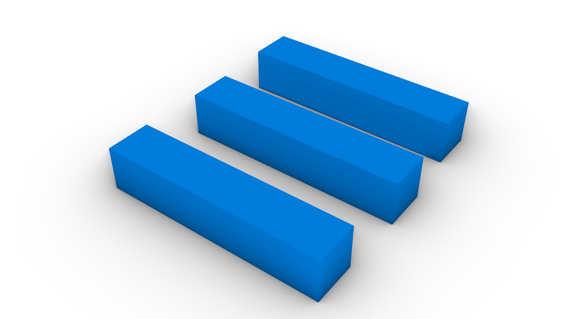
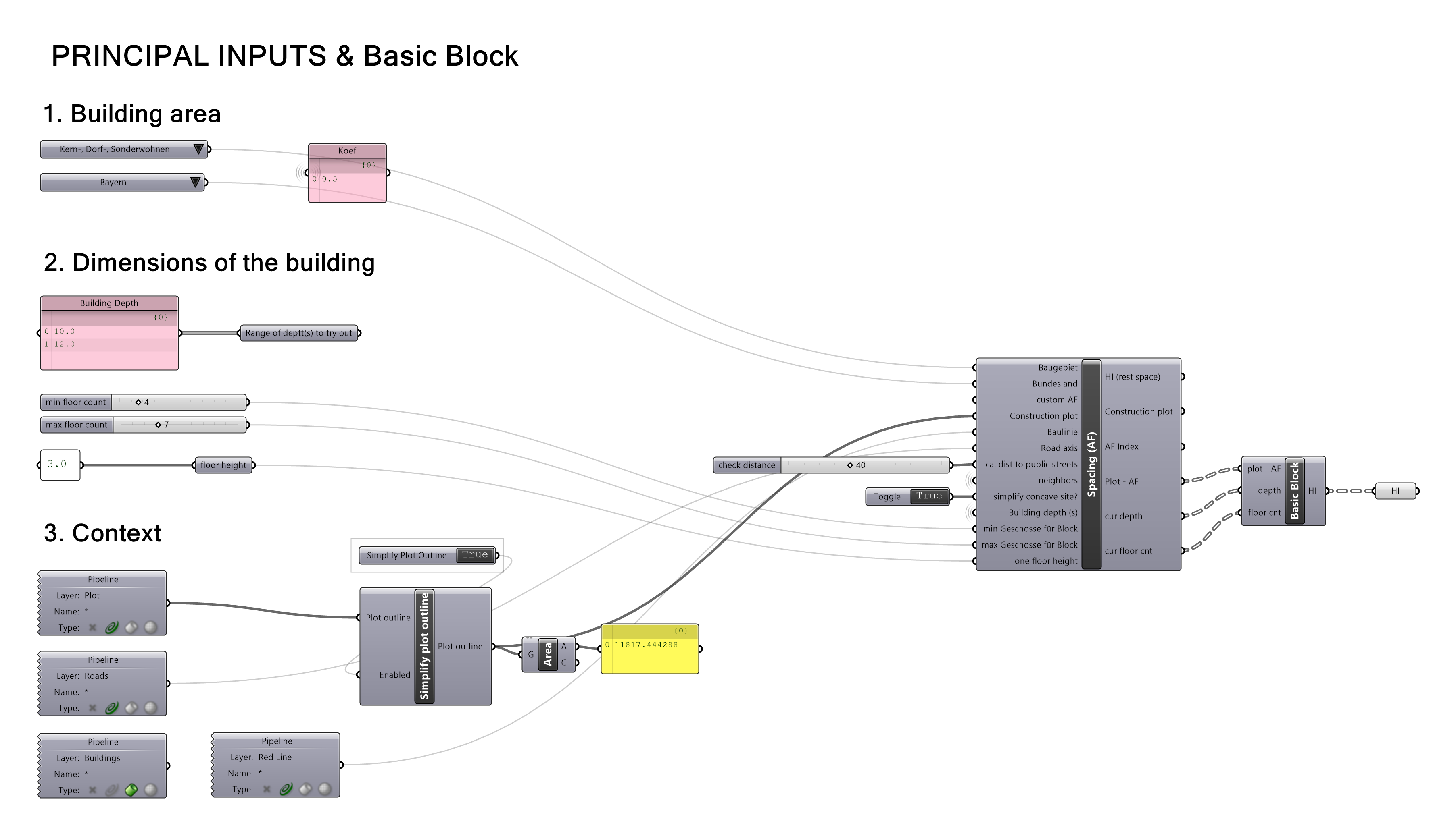
It is as well required to select the location of the building area in order to derive the correct spacing (see the video above to learn about the spacing concept). Further, you can select multiple values for the building depth to try out, as well as set up a range of the floors count for the basic block. The output of this step is a closed block (or a range of those) around the construction plot perimeter, considering the required spacing based on the block height.

It is possible though, that the spacing should be neglected, in case that your construction plot is placed within existing blocks and thus you should continue the street profile, placing the buildings right along the plot edge. In this case, you can just draw the lines in Rhino to indicate where the spacing should not appear, and insert them into ā€žBaulinieā€œ input.

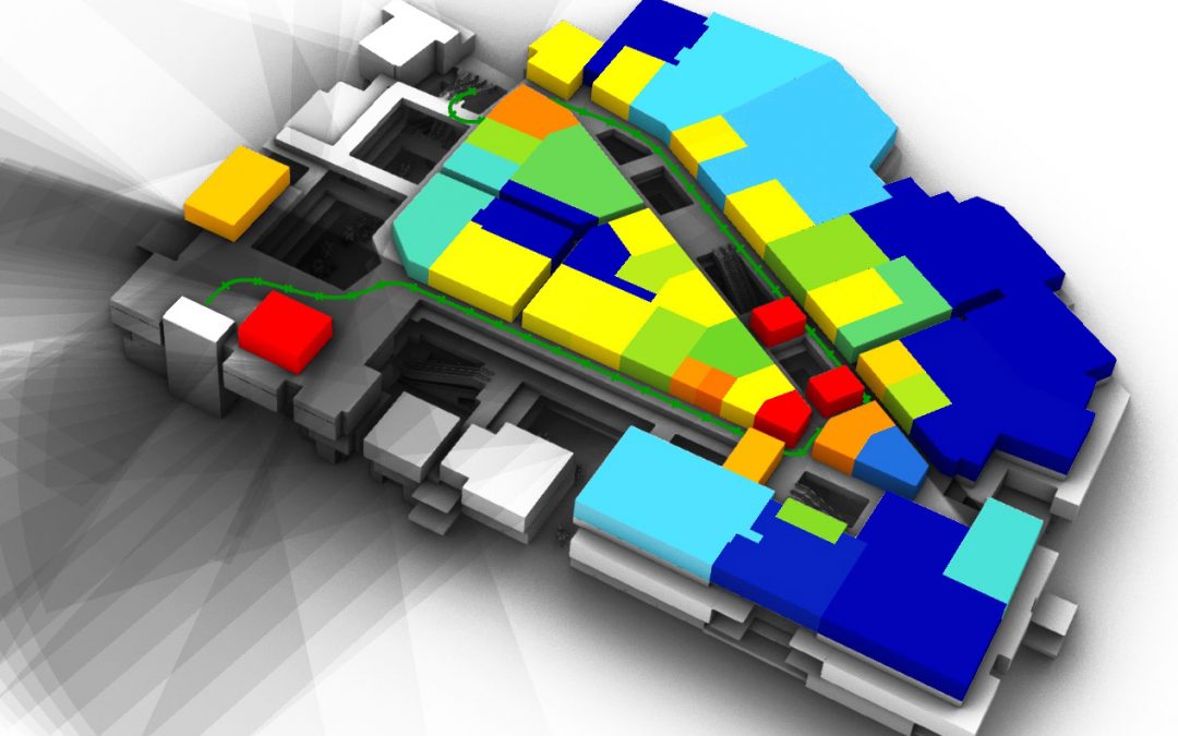
The resulting generations are gathered at the ā€žHouse Instanceā€œ data type, which is a combination of six different parameters: plot after spacing; surfaces; outlines (faƧade lines towards the street); inlines (faƧade lines towards towards the inner yard); depth of a building (as a number), floor count (as a number). Using Surface and Floor Count you can display the geometry preview as well as calculate the basic performance indicators, such as FAR, Site Occupancy, or Total Built Area.


1b. Actions over the Block.


1b.1| DELETE EDGES

This action can delete one or multiple edges to reduce the density or to solve a too narrow concave block intersection. You can select the edge to start with and decide on the number of edges to delete.


1b.3| SETBACKS CORNERS

This action creates a setback at the corner if the length of the adjusting edges is sufficient and the setback does not cause an intersection. You can select the edge for generation, dimensions range for the setback parameters and a seed for the randomness.


1b.5| CORNERBREAKS

This action creates passageways in the blockā€˜s corners, thus avoiding the creation of corners that are rather difficult for the later apartments placement. You can change the width of the passageways as well as the directions of the cuts.


1b.7| ENVELOPES

This action creates a spacing envelope, as well as both summer and winter solar envelopes (with the help of LadyBug tools). Informed by those envelopes, you can place buildings that act according to the local requirements, or that are placed to minimize the influence on the lighting conditions for the neighbor buildings around the given site.


Download Grasshopper file

1b.| YARD BUILDINGS

This action creates buildings within the block yard after the user-drawn axis. You can select the depth of the yard buildings as well as their floor count.


1b.2| SETBACKS EDGES

This action creates a setback along an edge if the edge length is sufficient. You can selecte the edge for generation, dimensions range for the setback parameters and a seed for the randomness.


1b.4 | RANDOM BREAKS

This action creates passageways through the block perimeter at either random, or user-driven spots. You can select the total amount of area to delete or the total width of the passageways, as well as the number of random options to try out per input block.


1b.6 | REDUCE HEIGHT

This action cuts the block through the corners and reduces the floor count of some of the building fragments. Here, you can indicate the total amount of area to delete. This actions creates several different height profiles per input block.


1b.8 | TOWERS

This action places one or two towers along the existing block perimeter in order to gain extra area. You can select the desired area per tower, restrict the extra floors, or assign a point where the tower should be located if you dont want random generations to appear. The limit of tower height is resulting from the envelopes script.


1b.10 | ROOFTOPS

This action creates offsetted rooftop floors over the block perimeter. You can decide on the orientation of the buildings (toward street/yard), depth, and their overall amount.


1c. Examplatory Generation Sequence

In the following video youā€˜ll find an examplatory combination of actions for generating a bunch of various building volumes for one construction site, including the parameters setting for each of the actions. Keep in mind that the suggested sequence is not the only possible one, and you can try to arrange actions in another way, and thus receive different results.


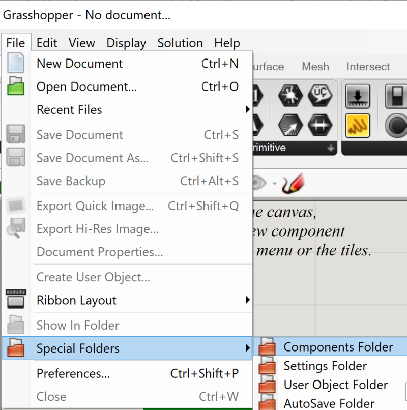
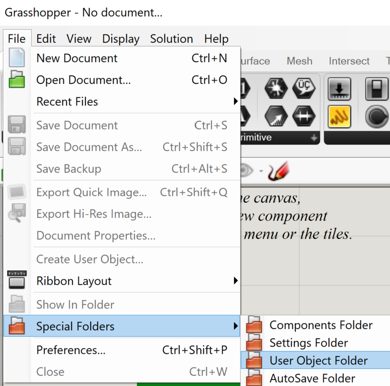
*please remember to unblock the .gha components before inserting them into your Libraries folder

Part 2:

Slabs Generation Components

2a. Single Plot Generation.

Here, the generation logic is slightly different than it was the case for the block typology. Whereas block was about offsetting and further modifying the site outline, slabs is about the pattern of the placement of several simple forms on the given site. Therefore, it is possible to order several slabs at one site. First, the site edges are translated into 4 characteristic edges based on the angles between them.

Further, slabs can appear along each of the edges ā€“ as long as the space is sufficient.


Depending on the selected order of the edges, the pattern of the slabs allocation can differ greatly.


Accordingly, each further parameter to influence the slabs pattern is repeated four times in order to allow different variations along each of the edges. In all further parameters, the order of the values will be applied accordingly to your selected order of the site edges. You can re-adjust the edges order at any later moment of the generation. Below, you can find a short video with the overview of the parameters that you can influence for the slabs typology.

2b. Subdivision of Complex Concave Sites and Multiple Plots Generation

In case of large area plots, such generation might cause monotonous strict patterns, non usable for modern urban plannings. In order to escape this, we developed a method on the subdivision of the big concave plots into smaller and simpler sub-fragments. Those sub-plots can then be filled with slabs in a single direction.

In the previous part, there were nine parameters for each slab raw at a single edge. In the case of generating slabs for multiple plots at the same time, the number of parameters gets multiplied accordingly. As follows, taking control over generation becomes exhausting. That is why for the multiple plots generation it was decided to leave only single-direction slabs. However, the user can decide between different orientation patterns as well as subdivision patterns himself, thus still exploring the design space to a several extent. In the following video you can see the brief overview of parameters to guide the generation for the slabs typology at multiple sites.

Tutorial | 2D and 3D isovists for visibility analysis

Tutorial | 2D and 3D isovists for visibility analysis

This tutorial demonstrates the use of 2d and 3d isovist components for the visibility analysis of architectural and urban space. The collection of example files presented in this blog post is part of the online course on visibility analysis from online teaching platform (OTP) forĀ  the Computational Methods in Architecture, Urban Design and Planning at Bauhuas University Weimar. The implementation of 2d isovist is based on the concepts presented by Benedikt in 1979. The 3d isovist was developed by the DeCodingSpaces team as extension of principles for constructing 2d isvovist to the third dimension. For further details on the isovist measures and the theory behind it, please visit the Bauhaus OTP platform.

Development team:

Martin Bielik 1,Ā  Ekaterina Fuchkina1, Sven Schneider1, Reinhard Koenig2,3

1Ā Bauhaus University, Weimar, Computer Science in Architecture
2 Bauhaus University, Weimar,Ā  Computational Architecture
3 Digital Resilient Cities, Austrian Institute of Technology

Credits:

Virtual Westgate 3D Model: Cognition, Perception, and Behaviour in Urban Environments, Future Cities Laboratory, Singapore-ETH Centre

Ā Li, H., Thrash, T., Hƶlscher, C., & Schinazi, V. R. (2019). The effect of crowdedness on human wayfinding and locomotion in a multi-level virtual shopping mall. Journal of Environmental Psychology, 65(January), 101320.


Topics covered in tutorial:

2D ISOVIST

  • single isovist
  • isovist along path
  • isovist field
  • results visualisation / object mapping

For all examples, we calculate following 2d isovist measures:

Area, Perimeter, Compactness, Circularity, Convex deficiency, Occlusivity, Min radial, Max radial, Mean radial, Standard deviation, Variance, Skewness, Dispersion, Elongation, Drift angle, Drift magnitude

3D ISOVIST

  • single isovist
  • isovist along path
  • isovist field
  • results visualisation / object mapping

For all examples, we calculate following 3d isovist measures:

Volume, Min radial, Max radial, Mean radial, Standard deviation, Sky factor, Ground factor, Object factor

Building context*


*the building geometry is subject of copyright and cannot be freely shared. The grasshopper scripts are free to download

Ā 

Requirements:

Install instructions:

Unblocking plugins

After downloading the DeCodingSpaces toolbox archive file, check if its unblocked before extracting the zip archive. Right click on the file > Properties > select unblock > select ok

Install components

After unlocking and extracting the DeCodingSpaces toolbox archive, copy the “DeCodingSpaces Libraries” folder into the grasshopper component folder. The grasshopper component folder can be found at:

C:\\Users\\YourUserName\\AppData\\Roaming\\Grasshopper\\Libraries

or via grasshopper file menu:

Install user objects

After unlocking and extracting the DeCodingSpaces toolbox archive, copy the “DeCodingSpaces UserObjects” folder into the grasshopper UserObjects folder. The grasshopper component folder can be found at:

Ā C:\\Users\\YourUserName\\AppData\\Roaming\\Grasshopper\\UserObjects

or via grasshopper file menu:

IMPORTANT NOTES:

1. Use only DeCodingSpaces toolbox version from this tutorial (see ling above). Any earlier or later version might cause errors.
2. GPU acceleration runs only on CUDA compatible graphic cards – NVIDIA GPU’s

Part 1:

2D isovist analysis

1a. Urban context

Start here, the urban examples are simple and easy to interact with. The observer as well as the obstacles (buildings) are positioned on flat plane. The urban examples do not require any external Rhino file to run. All geometry is already embedded in the grasshopper files.

1a.1| SINGLE ISOVIST

Basic setup the 2d isovist component. You can experiment with the view angle, direction, range parameters. Try to change the number of rays used to generate the isovist to speed up the calculation or increase the precision.


Download Grasshopper file

1a.3| ISOVIST PATH

Constructing directed 2d isovist along predefined path. Construct your own path through the environment and try different settings for view angle and view range. Observe how the isovist measures are changing during the movement along the path


Download Grasshopper file

1a.2| VISIBILITY MAPPING

Mapping the visibility back to the surrounding objects. We show how to map the results on the obstacle linesĀ  – building facades and buildings. We color the surrounding context based on its visibility. Additionally, we demonstrate how to normalize the visibility of objects by their length (for facades) or area (for buildings)


Download Grasshopper file

1a.4 | ISOVIST FIELD

Calculate 2d isovist properties for multiple vantage points arranged on the grid. Change the grid size and observe how the high and low values for each measure are distributed throughout the space.


Download Grasshopper file

1b. Building context

These are more advanced examples build on the same principles as show in the urban context section. The main reason adding extra complexity to the algorithms is the need to automatically filter the obstacle geometry relevant for each floor and than map the results back.


IMPORTANT NOTES:

  1. The architectural examples do require external Rhino file to run. Please download and open this prior to running any example from this section.
    2d_3d Isovsits _building.3dm
  2. 2d isovist cannot be analyzed for multiple floors at the same time. Each floor has to be analyzed individually.
  3. Algorithm performance dependsĀ  on the number of obstacles being analyzed. To speed up the analysis, simplify the scene and use GPU acceleration

1b.1| SINGLE ISOVIST

Basic setup the 2d isovist component. You can experiment with the view angle, direction, range parameters. Try to change the number of rays used to generate the isovist to speed up the calculation or increase the precision. Turn on and off layers which are used as view obstacles and observe the effect on the isovist.


Download Grasshopper file

1b.3| ISOVIST PATH

Constructing directed 2d isovist along predefined path through the different levels of the building. Construct your own path and try different settings for view angle and view range. Observe how the isovist measures are changing during the movement along the path.


Download Grasshopper file

1b.5 | ISOVIST FIELD

Calculate 2d isovist properties for multiple vantage points arranged on the grid. Change the grid size and observe how the high and low values for each measure are distributed throughout the space. View the results for individual floors.


Download Grasshopper file

1b.2| VISIBILITY MAPPING

Mapping the visibility back to the surrounding objects – shops. We show how to map the results on the obstacle linesĀ  – shopping windows and individual stores. We color the surrounding context based on its visibility. Additionally, we demonstrate how to normalize the visibility of objects by their length (for shopping windows) or area (for stores).


Download Grasshopper file

1b.4 | ISOVIST PATH CUMULATIVE MAPPING

Map the results from the whole isovist path on shops. View the results for individual floors.


Download Grasshopper file

1b.6 | VERTICAL ISOVIST

Calculate 2d isovist properties for section through the building. Since the 2d isovist is always calculated in XY plane, we rotate the building geometry by 90 degrees, calculate the isovist and rotate everything back. Move isovist vantage point through the building and see how the vertical 2d isovist changes. You can also define the view direction of the vertical 2d isovist plane.


Download Grasshopper file

Utilities

ANALYSIS GRID

Utility from DeCodignSpaces toolbox for automated generation of analysis grids. Define the analysis boundary, grid cell size and the area inside of which the grid should be generated.


Download Grasshopper file

Part 2:

3D isovist analysis

2a. Urban context

Start here, the urban example is simple and easy to interact with. The observer as well as the obstacles (buildings) are positioned on flat plane. The urban examples do not require any external Rhino file to run. All geometry is already embedded in the grasshopper files.

2a.1| SINGLE 3D ISOVIST

Basic setup the 3d isovist component. You can experiment with the horizontal and vertical view angle, direction, range parameters. Try to change the number of rays used to generate the isovist to speed up the calculation or increase the precision.


Download Grasshopper file

2b. Building context

These are more advanced examples for 3d isovist build on the same principles as show in the urban context section.


IMPORTANT NOTES:

  1. The architectural examples do require external Rhino file to run. Please download and open this prior to running any example from this section.
    2d_3d Isovsits _building.3dm
  2. Algorithm performance dependsĀ  on the number of obstacles being analyzed. To speed up the analysis, simplify the scene and use GPU acceleration

2b.1| SINGLE 3D ISOVIST

Basic setup the 3d isovist component. You can experiment with the horizontal and vertical view angle, direction, range parameters. Try to change the number of rays used to generate the isovist to speed up the calculation or increase the precision. Turn on and off layers which are used as view obstacles and observe the effect on the isovist.


Download Grasshopper file

2b.2| 3D ISOVIST PATH

Constructing 3d isovist along predefined path and map the visibility back to the surrounding objects – shops. We color the surrounding context based on its visibility. Additionally, we demonstrate how to normalize the visibility of objects by their length (for shopping windows) or area (for stores).


Download Grasshopper file

2b.3| 3D ISOVIST FIELD

Calculate 3d isovist properties for multiple vantage points arranged on the grid. Change the grid size and observe how the high and low values for each measure are distributed throughout the space. View the results for individual floors.


Download Grasshopper file

Urban Planning Table – Integrated Infrastructure

Urban Planning Table – Integrated Infrastructure

Video with impressions of the urban planning table, a walkthrough and created plans of all participants.

Introduction

Many different urban stakeholders such as authorities, planners, investors or local residents are involved in urban planning processes. Coordination and communication between the parties involved is often difficult, especially since not all parties have the same level of knowledge. This is particularly problematic when plans are not understood by those affected by the planning decisions.

The Ethiopian Ambassador in Germany (right) listens to our explanation of the project.

Ā As part of the research project “Integrated Infrastructure – IN3”, we want to support planning participants in developing Ethiopian villages into towns in tow ways. First, we create and discuss digital tools with the participants to enable fast urban planning. Second, we experiment with explanatory communication tools to provide village residents and local authorities with easy-to-use and game-like access to planning to enable conscious, participatory decision-making.

In a discussion with village representatives, we gained valuable insights using a prototypical communication tool. We drew attention to drastic changes in the village environment during a growth process from previous population of approx. 1,000 to the expected 10,000 inhabitants. This highlighted, for example, how land use and water infrastructure would be affected.

For the exhibition “įˆ įˆ‹įˆ Bauhaus” (Selam Bauhaus), we designed a simplified version that should give the users access to planning aspects in a fictious Ethiopian context without further help. The generated planning scenarios surely do not represent the final plans. We hope, however, that this type of interaction will stimulate discussion and reflection on new possibilities for planning and participation.

ā€œI believe that we need more knowledge and experience on town planningā€

ā€“ Villager

ā€œThe supportive maps and their relation to the existing context that you presented today are very interesting. We feel happy about the maps of our village that you [ā€¦] showed us. You showed us, how the growth and plans can affect our village.ā€

ā€“ Local representative

ā€œThis kind of planning is an improvement for our generation. We are in the 21st century and our aim is to give farmers and the rural community this opportunity of empowerment.ā€

ā€“ Local representative

User Experience

Being confronted with the complexities of planning and the multitude of challenges that arise, a user would be overwhelmed by the amount of information. Although the exhibited urban planning table simplifies planning relevant issues to estimatable and visualisable results, a direct confrontation with all parameters would lead to a visual clutter. Therefore, planning issues and population growth are introduced step by step with assisting information and contextutual visualisations:

1. Placement of city and setting its density – The city is small with a population of 1.000 inhabitants. The user has time to get used to the navigation and can move around the city through interaction with its icon.

2. Prioritising areas for agriculture or forest – The city grows to 3.000 inhabitants. A slider is introduced to weight the importance of nature against jobs in food production. The user can explore the difference not only on the map but also through performance evaluation.

3. Loss of agriculture demands new employment – The city has a population of 6.000 inhabitants. A new icon for industry is introduced. Moving it around affects air quality. Through two new sliders jobs in commercial or industrial sector can be created. It affects directly the land use plan of the city.

Exhibited Planning Table with an interactive map, the four planning steps on the bottom and performance evaluation on the upper right.

4. Satisfying water demand – The city reaches a population of 10.000 inhabitants. A water drop icons is now available and sets the location of a water tank. To reach water supply for every household the water pressure needs to be high enough and therefore the water tank should be placed on high altitude.

Finish. Based on the four steps, the user can simulate the population growth through usage of a slider. Within the exhibition, the final plan has been print out for the user by the tool.Ā 

The interaction with the planning table happens through intuitive touch commands and the user is continously informed on the feasability of the chosen city layout through real-time performance evaluation.

Rotate Camera
Camera Zoom
Move Camera
Move Objects
Performance Evaluation

Performance Evaluation

The urban planning table evaluates certain factors such as walkability, water demand, infrastructure affordability, air quality, employment and connection to nature to give continous feedback on planning relevant issues. The planning table users will realise that the factors are interrelated and a benefit for one criteria will challenge another. Therefore, the users will have to weight and compromise on their own demands. The criteria are explained in more detailled:


Walkability

In a city of short distances, the most important facilities can be reached quickly. The closer people live to each other, the easier it is to meet on foot. A round city would be ideal, but there are other factors that belong to a good city. So is it worth losing a bit of walkability for other qualities?


Nature

Sufficient green spaces are important in many ways. Forests in particular can improve air quality, protect soil from erosion and prevent rain from seeping into the ground too quickly. In addition, green spaces close to cities can also be used for recreation. However, they are also an important building material that requires space and time. So to what extend should forest be given space?


Employment

Agriculture cannot provide enough jobs for a growing population. New commercial and industrial land use can help here. If too few jobs are available, parts of the population will have to work in neighbouring cities or will not get a job. If too many are available, there is a danger that no one will be able to occupy them or that commuter traffic will be too high. With which mix of functions can a balanced employment be achieved?

Water & Affordability

In order to supply a city with water, physical rules need to be considered. If there is not enough water pressure at a tap, no water flows. The pressure results from the difference in height between tank and tap, accordingly a water tank should be located high and close enough to the city. Furthermore, the larger a city is, the more expensive the infrastructure becomes. A dense city is therefore often cheaper to maintain. Where is an optimal location for a water tank for an affordable and complete water supply?Ā 

Air Quality

A city with fresh air has good conditions to be a healthy city. However, industry produces dirty exhaust air, which is blown into the residential areas by the wind. The local weather has east and west winds, depending on the day. The wind is visualised by the smoke clouds. So how should industry be placed to avoid pollution of the city?


By combining hard factors calculated by the computer with soft factors evaluated in discussion rounds. People who know little about urban planning can be involved in the early stages of the planning process and gain important decision-making competencies. According to the feedback given to us, we will continue improving and extending our tools and hope to share the results in the near future.

1/18

Now I am wondering how it looks on the ground?

2/18

I like that this city has a lot of green! City, people and nature are in balance and the air quality is good! Like to LIVE HERE!

3/18

A very cool Project. It will be the future of design so that human have more time to think about details.

4/18

Richtig cool, aber Navigation mit zwei Fingern funktioniert nicht so richtig gut. Ansonstend spannend!

5/18

good air is the most important!

6/18

Being an Ethiopian myself i am sure that this would play a handy role through the process of achieving a responsible and responsive design our country needs.

7/18

Great stuff!

8/18

Gutes Tool, um strategisch denken zu lernen! Education?

9/18

Maybe we can extend the design table to mobile device.

10/18

very interesting simulation

11/18

Wonderful simulation ā™„ interactive+++ – More forest, less industry! Maybe some other employment options (services instead of industrial production? šŸ™‚ )

12/18

This table should have as many variables as it can (sanitary lines, electical, public areas etc.). Maybe make two versions easy (now) & hard for academics.

13/18

I like this one ā™„

14/18

sehr anschaulich!

15/18

šŸ™‚

16/18

shows consequences of planning directly

17/18

a very nice Simulation – also from an IT Perspective!

18/18

Ich finde das Programm fragwĆ¼rdig. Auf jeden Fall eine gute Lƶsung um schnell etwas geplant zu haben. Trotzdem finde ich, dass so eine Art zu planen gegen die RealitƤt stĆ¶ĆŸt. Bspw. wo bekomme ich das Wasser her? Wie kann ich das GrĆ¼ne unterhalten? Sind die Gegebenheiten dort fĆ¼r Industrie?… etc.

Acknowledgement

Integrated Infrastructure (INĀ³ –Ā uni-weimar.de/integrated-infrastructure) is an interdisciplinary international research project at the Bauhaus-UniversitƤt Weimar (BUW) and the Ethiopia Institute for Architecture, Building Construction and City Development (EiABC) working within the Emerging Cities Lab – Addis Ababa (ECL-AA).

The urban planning table is conceptualised and developed within the Integrated Infrastructure Research Team.
EiABC: Zegeye Cherenet, Tesfaye Hailu, Ephrem Gebremariam, Kirubel Nigussie, Metadel Selashi,Ā Bilisaf Teferri, Israel Tesfu
BUW: Andreas Aicher, Nicole Baron, Martin Dennemark, Philippe Bernd Schmidt, Sven Schneider

Interface design and programming of the planning table by Martin Dennemark

The project is funded by the Federal Ministry of Education and Research in Germany (BMBF), German Academic Exchange Service (DAAD) and German Aerospace Center (DLR).

Satellite imagery aquired through educational license fromĀ Ā© Planet Labs Inc. www.planet.com.


Evolving Configurational Properties

Evolving Configurational Properties

article published at 12th Space Syntax Symposium at Jiaotong University, Beijing, China

SIMULATING MULTIPLIER EFFECTS BETWEEN LAND USE AND MOVEMENT PATTERNS


Martin Bielik 1, Reinhard Koenig2,3 , Ekaterina Fuchkina1, Sven Schneider1, Abdulmalik Abdulmawla1

1Ā Bauhaus University, Weimar, Computer Science in Architecture
2 Bauhaus University, Weimar,Ā  Computational Architecture
3 Digital Resilient Cities, Austrian Institute of Technology

Abstract

In this paper, we introduce simulation framework for examining the effect of street network configuration on the evolution of the relationship between movement and land use allocation over time. The causal chain introduced in Space Syntax literature suggests that the potential generated by spatial configuration of a street network influences how people move and that these movement flows attract specific types of land uses. These land uses generate in turn additional movement creating an endless cycle of mutual interactions. In Space Syntax, this interaction between movement flow and land use is assumed to work in a positive feedback loop, multiplying the initial potentials given by a street network configuration. The practical consequence of this hypothetical assumption for the Space Syntax method is that the outcome of the feedback loop can be predicted as multiplication of the initial state and therefore doesnā€™t have to be simulated.
In this paper, we introduce a computational method for testing the multiplier effect hypothesis and identify the cases in which it holds true and those ones in which more detailed investigation considering feedback loops might be necessary. We demonstrate how such investigation based on the simulation of the interactions between movement and land use in time can be operationalized and conduct series of studies exploring the spatio-temporal effects of street network configuration.
We conclude that these exemplary studies show how the presented simulation model can be used to test the core assumption behind the Space Syntax method. We also offer preliminary insides about when and under which conditions it can be reliably applied and when system dynamic simulation might be necessary to predict not only the immediate, but also the long-term effects of street network configurations on centrality, movement and land use distribution.

Keywords

Street network configuration, System dynamics, Centrality, Movement, Land use, Multiplier effects, Natural movement


One sentence summary:

We explore the evolution of the configurational effects of urban form on the movement and land use allocation over time.

Paper overview

In this section, we compiled a short review of the main ideas discussed in the paper. The purpose is to get a general idea that can be deepened by reading the full paper attached below.

1. Background | What do we already know?

A)

ā€œStreet network configuration affects how people moveā€


(Golledge 1995)
B)

ā€œStreet network configuration affects where human activities allocateā€

(Hansen 1959)
C)

ā€œMovement influences allocation of land uses and allocation of land uses influence movementā€

(Hillier 1996a)

D)

ā€œSpace Syntax is about bringing the configuration, movement and allocation of activities togetherā€

(Hillier 1996b)

2. Research gap | What do we don’t know?

ā€œDoes the effect of street network configuration on movement and land use allocation evolve over time?ā€

OPTION A)

“The effect of configuration on movement and land use is stable over time, it DOES NOT EVOLVE

OPTION B)

“The effect of configuration on movement and land use does DOES EVOLVE over time”

Consequences

A) = SIMPLE TO PREDICT

B) = HARD TO PREDICT


Source: http://labs.minutelabs.io/Chaotic-Planets

3. Research question | What do we want to know?

Question A

Under which conditions is the result of the feedback loop between movement and land use distribution predictable as a function of the multiplier effect?

Ā 

Question B

Under which conditions does the natural movement potential of the network configuration correct the effect of unequal distribution of land uses (disruptions) throughout the feedback cycle?

Ā 

“Space Syntax method is based on the assumption that option A holds true. In other words, it is assumed that the outcome of the interaction between land use and movement can be predicted without simulation.”

This assumption is based on:

1. Multiplier effect hypothesis

The result of the feedback loop between movement and land use distribution is predictable as a function of the multiplier effect

(Hillier 1996b)
2. Natural movement hypothesis

The natural movement potential of the network configuration corrects the effect of unequal distribution of land uses (disruptions) throughout the feedback cycle

(Hillier 1999)

4. Research method | Spatio-temporal simulation engine

Left ) UML diagram of the Space Syntax underlying urban dynamics model. a) current model of the feedback loop between movement and land use. b) displays the ā€œmultiplier effectā€ hypothesis.
Right) Exemplary illustration of two iterations of our dynamic simulation. The initial state is an equally loaded network. The centrality values show the angular betweenness centrality with radius Rn (global radius).Value range: high movement potential = red, low movement potentialĀ  = blue

5. Results | Simulation experiments

We exemplary explore the impact of different conditions on the multiplier and natural movement effect. The conditions explored in this study relates to how we model the effect of land use on movement and what is the initial distribution of land use in the simulation.

Explored conditions & model parameters:

  • Definitions of movement potential centrality MPC.
    Closeness vs. Betweenness centrality
  • Analysis radius
    Local radius of 600m vs. global radius
  • Initial land use weightings w
    Equally loaded vs. Disrupted network*

For the following experiments, we used the street network of the inner city of Weimar as an exemplary case study area. Weimar is a medieval, mid-size German city with approximately 60.000 inhabitants. The size, historical development and the overall variety of street network patterns makes it a good candidate for testing the proposed simulation model. On the one hand, the size of the city makes it possible to quickly calculate many iterations of the simulation, but on the other hand it is large and diverse enough to let non-trivial configurational patterns emerge.

*Disrupted network in context of this paper means that in the initial stage of the simulation, not all street are loaded with equal amount of land use. In other words some streets produce more movement than others, which is represented by higher weighting of selected graph vertices.

Experiment 1 | Measuring the multiplier effectsĀ  on equally loaded network

Equally loaded network in context of this paper means that in the initial stage of the simulation, all street are loaded with equal amount of land use. In other words all streets produce same amount of movement, which is represented by equal weighting of all graph vertices.

E.1a

Conditions:

  • Equally loaded network
  • Betweenness centrality
  • Global radius
E.1c

Conditions:

  • Equally loaded network
  • Betweenness centrality
  • Local radius
E.1b

Conditions:

  • Equally loaded network
  • Closeness centrality
  • Global radius
E.1d

Conditions:

  • Equally loaded network
  • Closeness centrality
  • Local radius

Experiment 1 | Summary

Quantifying the multiplier effect by measuring linear relationship between the movement pattern at the first and the last iteration of the simulation


  • Multiplier effect is reliable predictor for:
    i) global closeness centrality
    ii) global betweenness centrality
  • Strong effect of scale of the centrality model
    Multiplier effect Global > Multiplier effect Local

Experiment 2 | Measuring the multiplier effects on disrupted network

Disrupted network in context of this paper means that in the initial stage of the simulation, not all street are loaded with equal amount of land use. In other words some streets produce more movement than others, which is represented by higher weighting of selected graph vertices.

E.2a

Conditions:

  • Disrupted network
  • Betweenness centrality
  • Global radius
E.2c

Conditions:

  • Disrupted network
  • Betweenness centrality
  • Local radius
E.2b

Conditions:

  • Disrupted network
  • Closeness centrality
  • Global radius
E.2d

Conditions:

  • Disrupted network
  • Closeness centrality
  • Local radius

Experiment 2 | Summary

Quantifying the multiplier effect by measuring linear relationship between the movement pattern at the first and the last iteration of the simulation


  • Multiplier effect is NOT reliable predictor
  • Doesnā€™t pick up most central streets*.* Non normality & heterocsedascity

Experiment 1&2 | Measuring the natural movement effect

Quantifying the natural movement effect by measuring linear relationship between the movement pattern at the first iteration of equally loaded network and last iteration of the disrupted network.


  • Natural movement is reliable predictor for:
    i) global closeness centrality

6. Conclusions | Joined multiplier and natural movement effect

Evaluating the impact of scale, initial network loading, and type of centrality measure on natural movement and multiplier effect. In other words, under which conditions is the influence of configuration on movement predictable without simulations and when the simulation is needed.


NO SIMULATION IS NEEDED:

  • For global closeness and betweenness centrality in equally loaded networks
  • For global closeness and in disrupted networks

SIMULATION IS REQUIRED:

  • When running local models
  • When running models on disrupted ā€“ non equally loaded networks

7. Outlook | Next steps

A) Testing the simulation results against empirical longitudinal data

B) Testing the sensitivity of multiplier and natural movement effect on conditions related to street network configuration and type of land use (i.e. does multiplier effect depends on the type of the street network layout and how we model the impact of movement on land use).


Download the article

Bielik et al. – 2019 – Evolving configurational properties.pdf


Cite the article

Bielik, M., Koenig, R., Fuchkina, E., Schneider, S., & Abdulmalik, A. (2019). EVOLVING CONFIGURATIONAL PROPERTIES – Simulating multiplier effects between land use and movement patterns. Presented at the 12th Space Syntax Symposium, Beijing, China.
Ā 

Supplementary materials


Grasshopper scripts

Following grasshopper scriptĀ  simulates the interaction between movement flows and land use distribution through street network configuration. The street network used in the example is simplified example of city of Weimar, Germany which was used as an example in the paper. The data for the street network is directly embedded in this script.

Versions of the script:

1. Simplified script, easy to run. This script requires only DeCodingSpaces toolbox and Anemone plugins being installed (see instructions bellow)
evolving configurational properties_simple.gh

2. Full script. This script requires also R language additionally to DeCodingSpaces toolbox and Anemone plugins being installed (see instructions bellow). This version of the script offers some additional visualization and possibility to save the simulation results
evolving configurational properties_full.gh


NOTE: Get sure the GPU acceleration is enabled.
(otherwise is the simulation too slow to execute in real time)
NOTE: Check the requirements section bellow and get sure you get all the plugins installed using the links on this website.(otherwise the version might not fit the version of the script)


Requirements

Install instructions

Unblocking plugins

After downloading the RequiredGHPlugins_SimAUD19.zip file, check if its unblocked before extracting the zip archive. Right click on the file > Properties > select unblock > select ok

Install components

After unlocking and extracting the RequiredGHPlugins_SimAUD19.zip archive, copy the “SimAUD19 components” folder into the grasshopper component folder. The grasshopper component folder can be found at:

 C:\Users\YourUserName\AppData\Roaming\Grasshopper\Libraries

or via grasshopper file menu:

Install user objects

After unlocking and extracting the RequiredGHPlugins_SimAUD19.zip archive, copy the “SimAUD19 user objects” folder into the grasshopper UserObjects folder. The grasshopper component folder can be found at:

 C:\Users\YourUserName\AppData\Roaming\Grasshopper\UserObjects

or via grasshopper file menu:

Enable GPU acceleration

The requirement to run the GPU accelerated street network analysis is the CUDA platform enabled NVIDIA GPU.
If this requirement is fulfilled, you have to copy the folders ā€œAlea.CUDA.CT.LibDeviceā€ and ā€œAlea.CUDA.CT.Native.X86.B64.Windowsā€ from the GPU acceleration folder to your Rhino install folder (i.e. ā€œProgram Files\Rhinoceros 6 (64-bit)\System\ā€).

SSS12 Workshop | Parametric urban planning with Space Syntax and DeCodingSpaces-toolbox for Grasshopper

SSS12 Workshop | Parametric urban planning with Space Syntax and DeCodingSpaces-toolbox for Grasshopper

The workshop onĀ parametric urban planning Ā with Space Syntax and DeCodingSpaces-toolbox for Grasshopper is hosted by:

The 12th International Space Syntax Symposium (12SSS) will be held in Beijing from 8th to 13th July 2019, at Beijing Jiaotong University


Lecturers:

Reinhard KƶnigĀ  Ā Ā Ā Ā Ā Ā Ā Ā Ā Ā Ā Ā Ā Ā Ā Ā  Bauhaus University, Weimar
Martin BielikĀ Ā Ā Ā Ā Ā Ā Ā Ā Ā Ā Ā Ā Ā Ā Ā Ā Ā Ā Ā Ā Ā  Bauhaus University, Weimar
Yufan Miao Ā Ā Ā Ā Ā Ā Ā Ā Ā Ā Ā Ā Ā Ā Ā Ā Ā Ā Ā Ā Ā Ā Ā Ā  ETH Zurich, FCL Singapore

Short summary:

During this one-day-workshop you will be introduced to methods for the analysis, generation and optimizations of urban layouts with DeCodingSpaces-Toolbox for Grasshopper. We will use existing urban context to analyze the impact of the street network configuration on different types of human behavior such as movement, walkability or land use distribution. Than we will learn how to use the analysis results to generate new street network layouts, parcels and buildings parametrically. Finally, we will demonstrate how to you evolutionary optimization to improve the performance of the parametric design toward pre-defined planning goals.

For this purpose we use Grasshopper for Rhino3D with the plugin DecodingSpaces-Toolbox. The methods are demonstrated by realistic case studies in an existing urban environments.

This workshop is intended for both practitioners and researchers interested in rapid context aware generation of urban layouts. The presented workflow let you computationally explore the design options of new urban development area with the potential to assess the site potential and inform the early planning stages.

Workshop schedule

8:30 – 9:00 Registration
9:00 – 12:25 Analysis | Street network analysis with DeCodingSpaces Toolbox

Shortest paths – Metric, Angular, Custom
Multi modal travel
Centrality measures
Weighting origins and destinations of movement
12:25 – 13:30 Lunch break
13:30 – 15:00 Generation | Parametric urban form synthesis

Street network synthesis
Street block recognition
Parametric parcelation
Parametric building generation
15:00 – 15:30 break
15:30 – 17:00

Optimization | Evolutionary optimization of street network configuration

Evolutionary optimization basics
Street network as custom chromosome
Application examples

Install instructions

Unblocking plugins

After downloading the RequiredGHPlugins_SimAUD19.zip file, check if its unblocked before extracting the zip archive. Right click on the file > Properties > select unblock > select ok

Install components

After unlocking and extracting the RequiredGHPlugins_SimAUD19.zip archive, copy the “SimAUD19 components” folder into the grasshopper component folder. The grasshopper component folder can be found at:

 C:\Users\YourUserName\AppData\Roaming\Grasshopper\Libraries

or via grasshopper file menu:

Install user objects

After unlocking and extracting the RequiredGHPlugins_SimAUD19.zip archive, copy the “SimAUD19 user objects” folder into the grasshopper UserObjects folder. The grasshopper component folder can be found at:

 C:\Users\YourUserName\AppData\Roaming\Grasshopper\UserObjects

or via grasshopper file menu:

Enable GPU acceleration

The requirement to run the GPU accelerated street network analysis is the CUDA platform enabled NVIDIA GPU.
If this requirement is fulfilled, you have to copy the folders ā€œAlea.CUDA.CT.LibDeviceā€ and ā€œAlea.CUDA.CT.Native.X86.B64.Windowsā€ from the GPU acceleration folder to your Rhino install folder (i.e. ā€œProgram Files\Rhinoceros 6 (64-bit)\System\ā€).

Part 1 – Street Network Analysis

Presentation

Documentation

Interactive documentation of the Street Network Analysis toolbox.

Hands on example files:

Street Network Editing Utilities

01| CITY GRAPH STARTING EXAMPLE

Basic setup for different options how to use the street network analysis tools to calculate shortest paths and centrality measures.


Download Grasshopper file

04| CITY GRAPH ONE WAY ROADS

The underlying spatial graph is directed one, which means that to every street we can assign different distance weight in each direction. In the example we demonstrate how this can be used to model traffic regulation such as one way streets.


Download Grasshopper file

02| PARK EDGE WEIGHTING

Calculating shortest paths by assigning custom distance weights (graph edges) to the spatial network. The edge weights can be metric, angular, custom or any combination of these. Thus we can represent different concepts of distance (e.g. time, safety, cognitive distance)


Download Grasshopper file

05| CITY GRAPH CENTRALITY VERTEX WEIGHTING

When calculation street network centrality, we can assign custom weight to each graph vertex (origin and destination of shortest path). This can be used to model network in which some nodes (e.g. train station) produce more movement than others.


Download Grasshopper file

03| CITY GRAPH BUS EDGE WEIGHTING

The application of custom distance weights (edge weights) is demonstrated on the example of multi-modal transportation network. Street segment which serve as bus routes are given shorter distance representing travel time compared to pedestrian street segments.


Download Grasshopper file
Download Rhino file

06| CITY GRAPH CENTRALITY DISTANCE DECAY

In several centrality measures (e.g. gravity), the attractiveness of destination isĀ  inversely proportional to function of distance. As distance grows, the attractiveness is getting lower. In the street network analysis toolbox, this distance decay function can be defined by user representing different types of behavior and aversion to travel.


Download Grasshopper file

Street Network Editing Utilities

01| NETWORK EDITING TOOLS

To gain correct and speedy analysis results of any street network, this has to be usually simplified and corrected for drawing errors. DeCodingSpaces toolbox offers range of tools to split lines, remove duplicates, simplify intersections and remove dead ends.


Download Grasshopper file

02| CUSTOM OFFSET

Transforms the street network into closed polylines – street blocks which can be offseted by custom value for each block edge. We demonstrate this functionality by offseting the block edges by their respective street network centrality values.


Download Grasshopper file

Part 2 – Generation of Street network, Plots and Buildings

Street Network Optimization

01| STREET NETWORK GENERATION

Generate Street Networks in a given area with initial street segments by controlling parameters for street segment length, angle between streets and connectivity.


Download Grasshopper file

02| BUILDING PLOTS GENERATION

Based on the generated Street Network we extract the Street Blocks and generate Plots based on control parameters like the maximal area, minimal width of the street side, etc.


Download Grasshopper file

03| BUILDING GENERATION

For each plot we generate buildings of various typologies controlling the parameters for setbacks, building sizes, orientation and density.


Download Grasshopper file

Part 3 – Street Network Optimization

Hands on example files:

Street Network Optimization

01| Chromosome Demonstration

In this example file, we demonstrate how the generative methods are represented using a specific data structure to be used for evolutionary optimization in the next step.


Download Grasshopper file

02| Evolutionary Multi-Criteria Optimization

Based on the generative components and a particular data structure, we can use a multi-criteria evolutionary optimization algorithm to search for good urban design variants.


Download Grasshopper file

SimAUD 2019 Workshop | Adaptive Urban Layout Optimization with DeCodingSpaces-Toolbox

SimAUD 2019 Workshop | Adaptive Urban Layout Optimization with DeCodingSpaces-Toolbox

During this one-day-workshop you will be introduced to methods for the analysis, synthesis and optimization of urban layouts. We will cover computational generation of the street network, parcellation and the building form, based on the existing urban context and various design goals. You learn how to analyze street networks effectively, and we show you how to compare and optimize the generated designs systematically. For this purpose we use Grasshopper for Rhino3D with the plugin DecodingSpaces-Toolbox, and a new Design-Space-Exploration tool. The methods are demonstrated by realistic case studies in an existing urban environments.

This workshop is intended for both practitioners and researchers interested in rapid context aware generation of urban layouts. The presented workflow let you computationally explore the design options of new urban development area with the possibility to assess the site potential and inform the early planning stages. The presented DeCodingSpaces-Toolbox for Grasshopper is a collection of analytical and generative components for algorithmic architectural and urban planning. The toolbox is free software released by the Computational Planning Group (CPlan).

The workshop on Adaptive Urban Layout Optimization in Grasshopper is hosted by:

SimAUD 2019, Atlanta – USA, School of Architecture, Georgia Tech,Ā  7. April 2019

Requirements

Install instructions

Unblocking plugins

After downloading the RequiredGHPlugins_SimAUD19.zip file, check if its unblocked before extracting the zip archive. Right click on the file > Properties > select unblock > select ok

Install components

After unlocking and extracting the RequiredGHPlugins_SimAUD19.zip archive, copy the “SimAUD19 components” folder into the grasshopper component folder. The grasshopper component folder can be found at:

 C:\Users\YourUserName\AppData\Roaming\Grasshopper\Libraries

or via grasshopper file menu:

Install user objects

After unlocking and extracting the RequiredGHPlugins_SimAUD19.zip archive, copy the “SimAUD19 user objects” folder into the grasshopper UserObjects folder. The grasshopper component folder can be found at:

 C:\Users\YourUserName\AppData\Roaming\Grasshopper\UserObjects

or via grasshopper file menu:

Enable GPU acceleration

The requirement to run the GPU accelerated street network analysis is the CUDA platform enabled NVIDIA GPU.
If this requirement is fulfilled, you have to copy the folders ā€œAlea.CUDA.CT.LibDeviceā€ and ā€œAlea.CUDA.CT.Native.X86.B64.Windowsā€ from the GPU acceleration folder to your Rhino install folder (i.e. ā€œProgram Files\Rhinoceros 6 (64-bit)\System\ā€).

Part 1 – Street Network Analysis

Presentation

Documentation

Interactive documentation of the Street Network Analysis toolbox.

Hands on example files:

Street Network Editing Utilities

01| CITY GRAPH STARTING EXAMPLE

Basic setup for different options how to use the street network analysis tools to calculate shortest paths and centrality measures.


Download Grasshopper file

04| CITY GRAPH ONE WAY ROADS

The underlying spatial graph is directed one, which means that to every street we can assign different distance weight in each direction. In the example we demonstrate how this can be used to model traffic regulation such as one way streets.


Download Grasshopper file

02| PARK EDGE WEIGHTING

Calculating shortest paths by assigning custom distance weights (graph edges) to the spatial network. The edge weights can be metric, angular, custom or any combination of these. Thus we can represent different concepts of distance (e.g. time, safety, cognitive distance)


Download Grasshopper file

05| CITY GRAPH CENTRALITY VERTEX WEIGHTING

When calculation street network centrality, we can assign custom weight to each graph vertex (origin and destination of shortest path). This can be used to model network in which some nodes (e.g. train station) produce more movement than others.


Download Grasshopper file

03| CITY GRAPH BUS EDGE WEIGHTING

The application of custom distance weights (edge weights) is demonstrated on the example of multi-modal transportation network. Street segment which serve as bus routes are given shorter distance representing travel time compared to pedestrian street segments.


Download Grasshopper file
Download Rhino file

06| CITY GRAPH CENTRALITY DISTANCE DECAY

In several centrality measures (e.g. gravity), the attractiveness of destination isĀ  inversely proportional to function of distance. As distance grows, the attractiveness is getting lower. In the street network analysis toolbox, this distance decay function can be defined by user representing different types of behavior and aversion to travel.


Download Grasshopper file

Street Network Editing Utilities

01| NETWORK EDITING TOOLS

To gain correct and speedy analysis results of any street network, this has to be usually simplified and corrected for drawing errors. DeCodingSpaces toolbox offers range of tools to split lines, remove duplicates, simplify intersections and remove dead ends.


Download Grasshopper file

02| CUSTOM OFFSET

Transforms the street network into closed polylines – street blocks which can be offseted by custom value for each block edge. We demonstrate this functionality by offseting the block edges by their respective street network centrality values.


Download Grasshopper file

Part 2 – Street Network Synthesis

Hands on example files:

Street Network Generation and Optimization

01| STREET NETWORK SYNTHESIS

02| Chromosome Demonstration

03| Evolutionary Multi-Criteria Optimization

In case you have issues with the Selector component of the DeCodingSpaces-Toolbox, it may be caused by the decimal symbol used by your operating system: make sure you use point, no comma. Second, ensure that the path to your PISA folder (part of the DeCodingSpaces-Toolbox in your libraries folder) has no space characters, points, or other special characters. You can copy the PISA folder with its content to C:\PISA and delete it from the libraries folder.

Part 3 – Exploration

Pin It on Pinterest