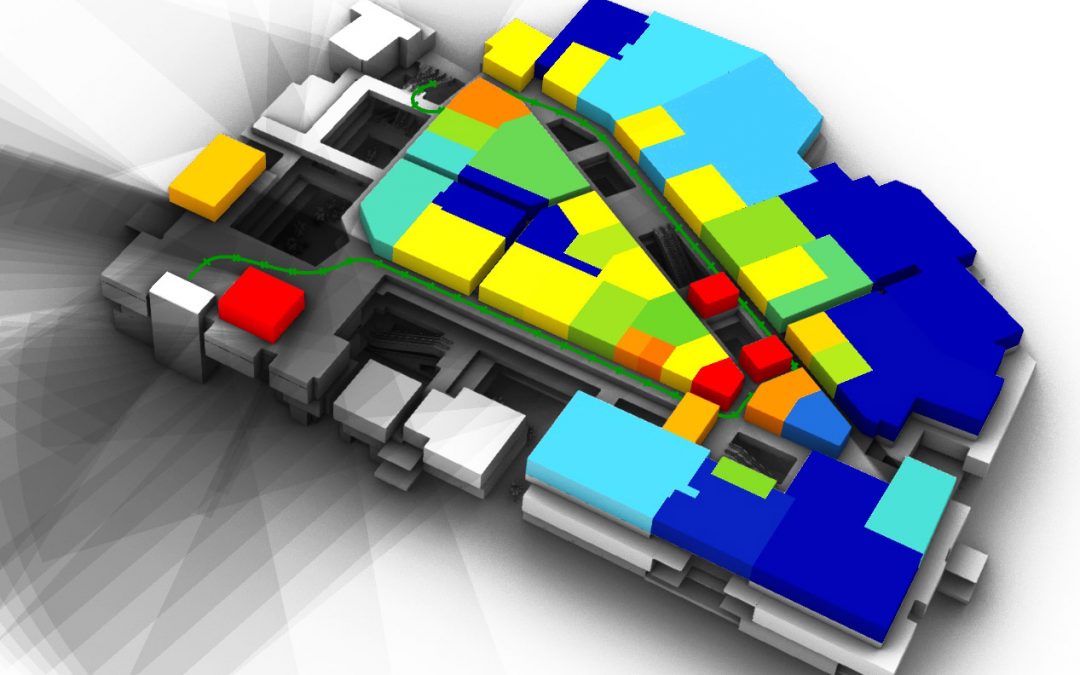
This tutorial demonstrates the use of 2d and 3d isovist components for the visibility analysis of architectural and urban space. The collection of example files presented in this blog post is part of the online course on visibility analysis from online teaching platform (OTP) for the Computational Methods in Architecture, Urban Design and Planning at Bauhuas University Weimar. The implementation of 2d isovist is based on the concepts presented by Benedikt in 1979. The 3d isovist was developed by the DeCodingSpaces team as extension of principles for constructing 2d isvovist to the third dimension. For further details on the isovist measures and the theory behind it, please visit the Bauhaus OTP platform.
Development team:
Martin Bielik 1, Ekaterina Fuchkina1, Sven Schneider1, Reinhard Koenig2,3
1 Bauhaus University, Weimar, Computer Science in Architecture
2 Bauhaus University, Weimar, Computational Architecture
3 Digital Resilient Cities, Austrian Institute of Technology
Credits:
Virtual Westgate 3D Model: Cognition, Perception, and Behaviour in Urban Environments, Future Cities Laboratory, Singapore-ETH Centre
Li, H., Thrash, T., Hölscher, C., & Schinazi, V. R. (2019). The effect of crowdedness on human wayfinding and locomotion in a multi-level virtual shopping mall. Journal of Environmental Psychology, 65(January), 101320.
Topics covered in tutorial:
2D ISOVIST
- single isovist
- isovist along path
- isovist field
- results visualisation / object mapping
For all examples, we calculate following 2d isovist measures:
Area, Perimeter, Compactness, Circularity, Convex deficiency, Occlusivity, Min radial, Max radial, Mean radial, Standard deviation, Variance, Skewness, Dispersion, Elongation, Drift angle, Drift magnitude
3D ISOVIST
- single isovist
- isovist along path
- isovist field
- results visualisation / object mapping
For all examples, we calculate following 3d isovist measures:
Volume, Min radial, Max radial, Mean radial, Standard deviation, Sky factor, Ground factor, Object factor


*the building geometry is subject of copyright and cannot be freely shared. The grasshopper scripts are free to download

Install instructions:
Unblocking plugins
After downloading the DeCodingSpaces toolbox archive file, check if its unblocked before extracting the zip archive. Right click on the file > Properties > select unblock > select ok

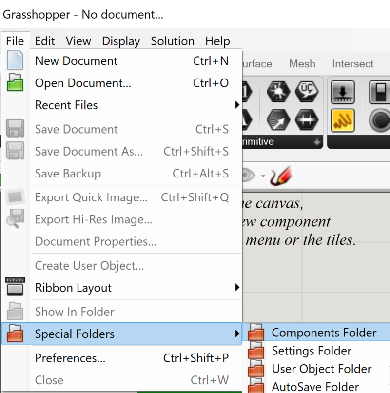
Install components
After unlocking and extracting the DeCodingSpaces toolbox archive, copy the “DeCodingSpaces Libraries” folder into the grasshopper component folder. The grasshopper component folder can be found at:
C:\\Users\\YourUserName\\AppData\\Roaming\\Grasshopper\\Libraries
or via grasshopper file menu:
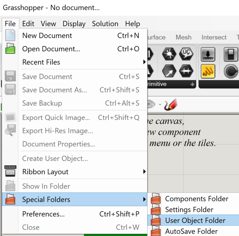
Install user objects
After unlocking and extracting the DeCodingSpaces toolbox archive, copy the “DeCodingSpaces UserObjects” folder into the grasshopper UserObjects folder. The grasshopper component folder can be found at:
C:\\Users\\YourUserName\\AppData\\Roaming\\Grasshopper\\UserObjects
or via grasshopper file menu:
IMPORTANT NOTES:
1. Use only DeCodingSpaces toolbox version from this tutorial (see ling above). Any earlier or later version might cause errors.
2. GPU acceleration runs only on CUDA compatible graphic cards – NVIDIA GPU’s
Part 1:
2D isovist analysis
1a. Urban context
Start here, the urban examples are simple and easy to interact with. The observer as well as the obstacles (buildings) are positioned on flat plane. The urban examples do not require any external Rhino file to run. All geometry is already embedded in the grasshopper files.

1a.1| SINGLE ISOVIST
Basic setup the 2d isovist component. You can experiment with the view angle, direction, range parameters. Try to change the number of rays used to generate the isovist to speed up the calculation or increase the precision.

1a.3| ISOVIST PATH
Constructing directed 2d isovist along predefined path. Construct your own path through the environment and try different settings for view angle and view range. Observe how the isovist measures are changing during the movement along the path

1a.2| VISIBILITY MAPPING
Mapping the visibility back to the surrounding objects. We show how to map the results on the obstacle lines – building facades and buildings. We color the surrounding context based on its visibility. Additionally, we demonstrate how to normalize the visibility of objects by their length (for facades) or area (for buildings)

1a.4 | ISOVIST FIELD
Calculate 2d isovist properties for multiple vantage points arranged on the grid. Change the grid size and observe how the high and low values for each measure are distributed throughout the space.
1b. Building context
These are more advanced examples build on the same principles as show in the urban context section. The main reason adding extra complexity to the algorithms is the need to automatically filter the obstacle geometry relevant for each floor and than map the results back.
IMPORTANT NOTES:
- The architectural examples do require external Rhino file to run. Please download and open this prior to running any example from this section.
2d_3d Isovsits _building.3dm - 2d isovist cannot be analyzed for multiple floors at the same time. Each floor has to be analyzed individually.
- Algorithm performance depends on the number of obstacles being analyzed. To speed up the analysis, simplify the scene and use GPU acceleration

1b.1| SINGLE ISOVIST
Basic setup the 2d isovist component. You can experiment with the view angle, direction, range parameters. Try to change the number of rays used to generate the isovist to speed up the calculation or increase the precision. Turn on and off layers which are used as view obstacles and observe the effect on the isovist.

1b.3| ISOVIST PATH
Constructing directed 2d isovist along predefined path through the different levels of the building. Construct your own path and try different settings for view angle and view range. Observe how the isovist measures are changing during the movement along the path.

1b.5 | ISOVIST FIELD
Calculate 2d isovist properties for multiple vantage points arranged on the grid. Change the grid size and observe how the high and low values for each measure are distributed throughout the space. View the results for individual floors.

1b.2| VISIBILITY MAPPING
Mapping the visibility back to the surrounding objects – shops. We show how to map the results on the obstacle lines – shopping windows and individual stores. We color the surrounding context based on its visibility. Additionally, we demonstrate how to normalize the visibility of objects by their length (for shopping windows) or area (for stores).
1b.4 | ISOVIST PATH CUMULATIVE MAPPING
Map the results from the whole isovist path on shops. View the results for individual floors.

1b.6 | VERTICAL ISOVIST
Calculate 2d isovist properties for section through the building. Since the 2d isovist is always calculated in XY plane, we rotate the building geometry by 90 degrees, calculate the isovist and rotate everything back. Move isovist vantage point through the building and see how the vertical 2d isovist changes. You can also define the view direction of the vertical 2d isovist plane.
Utilities
ANALYSIS GRID
Utility from DeCodignSpaces toolbox for automated generation of analysis grids. Define the analysis boundary, grid cell size and the area inside of which the grid should be generated.
Part 2:
3D isovist analysis
2a. Urban context
Start here, the urban example is simple and easy to interact with. The observer as well as the obstacles (buildings) are positioned on flat plane. The urban examples do not require any external Rhino file to run. All geometry is already embedded in the grasshopper files.
2a.1| SINGLE 3D ISOVIST
Basic setup the 3d isovist component. You can experiment with the horizontal and vertical view angle, direction, range parameters. Try to change the number of rays used to generate the isovist to speed up the calculation or increase the precision.
2b. Building context
These are more advanced examples for 3d isovist build on the same principles as show in the urban context section.
IMPORTANT NOTES:
- The architectural examples do require external Rhino file to run. Please download and open this prior to running any example from this section.
2d_3d Isovsits _building.3dm - Algorithm performance depends on the number of obstacles being analyzed. To speed up the analysis, simplify the scene and use GPU acceleration
2b.1| SINGLE 3D ISOVIST
Basic setup the 3d isovist component. You can experiment with the horizontal and vertical view angle, direction, range parameters. Try to change the number of rays used to generate the isovist to speed up the calculation or increase the precision. Turn on and off layers which are used as view obstacles and observe the effect on the isovist.

2b.2| 3D ISOVIST PATH
Constructing 3d isovist along predefined path and map the visibility back to the surrounding objects – shops. We color the surrounding context based on its visibility. Additionally, we demonstrate how to normalize the visibility of objects by their length (for shopping windows) or area (for stores).

2b.3| 3D ISOVIST FIELD
Calculate 3d isovist properties for multiple vantage points arranged on the grid. Change the grid size and observe how the high and low values for each measure are distributed throughout the space. View the results for individual floors.
perfect, thanks you very much, i am student, I am also research them
Hello sir ,
can the isovist field take a surface analysis a terrain surface with slopes ?
I tried it but couldn’t get it work,looks like it only accept flat terrain
Hey ,
does the isovist3D filed detects terrain with slope as obstacles ?
Hi, yes this should work!
Hello.
How do i sign up to download the building file?
Hi Moses, I am sorry but the building file is unfortunately subject to copyright and cannot be shared.
You have created a great toolbox. May I ask, how can I get the mesh output to work in 3D isovist? I am getting an invalid mesh, or null output..
Hi. May I know how do I sign up to download the building file?
Hi Bryan, I am sorry but the building file is unfortunately subject to copyright and cannot be shared.
How do i sign up to download the building file?
Hello! I’m trying to download the external Rhino files, but I get a 401 error page. A login and password are asked. How can I proceed?
Hi,
unfortunately, we are not allowed to share the building model publically, sorry.
Best regards
Reinhard
Hi, Can’t download any files. Help me
This happens to some users. Have you tried with the right mouse click – save as? Or try another browser. When I test it, it works fine.
Best regards
Reinhard
HI.I can’t download any files too.Also have changed the browsers either
Hi, I am a student. I’m very glad that you can share such excellent cases. Could you please package your case files and send them to my email address?
where can I get Cample Grasshopper data?
Hi- I’m wondering how well this works on topographic, grade oriented environments.
Say you have an urban environment on a slope, would you be able to traverse grades and make reasonable outcomes?
For some reason I am unable to download the example files… Is there anywhere I can access them?
hello, please help me to access the rhino file …
Hi, is there any tutorial of doing it??